Monte Carlo Options Pricing

December 17, 2021

The options casino

Predicting the movement of stock prices is an alluring challenge with the promise of riches. Unfortunately, predicting future stock prices consistently and reliably is generally considered impossible. However, we can use models to make useful predictions, manage risk, and profit probalistically.

Geometric Brownian Motion

One such commonly used model is geometric Brownian motion (1, 2) - in fact, the famous Black-Scholes options pricing formula assumes this model as well. This has the form

$$ \begin{align} S(t) = S(0)\exp{((\mu-\frac{\sigma^2}{2})t + \sigma B(t))} \tag{0} \label{eq:gbm} \end{align} $$

where $B(t)$ is standard Brownian motion. If we let $S(0)$ to be the initial stock price, $\mu$ to be the mean compounding return, and $\sigma$ to be the volatility of a stock, then we can generate very realistic price paths.

$\mu$ 0

$\sigma$ 0

So, what does this mean, and why is this a good model for security prices?

Logarithmic Returns

In quantitative finance it is common to deal with continuously compounded returns rather than simple returns. What that means is that instead of examining a simple return between trading periods $1 + R_t = \frac{S(t)}{S(t-1)}$ we will examine the compounding return $r_t = \ln{(1 + R_t)} = \ln{\frac{S(t)}{S(t-1))}}$. This has the very nice property that one can recover the price of a stock by simply summing up the logarithmic returns as:

$$ \begin{align} S(t) = S(0)\exp{(r_1 + r_2 + ... + r_{t-1})} \tag{1} \label{eq:rr} \end{align} $$

This is also convenient because a common assumption in finance is that the logarithmic returns of a stock are independent and normally distributed with mean $\mu$ and variance $\sigma^2$. Note that for small returns, simple returns $R_t$ approximate logarthmic returns $r_t$ since $r_t = \ln{(1 + R_t)} \approx R_t$, so the difference between the two returns is not substantial, and thus one can assume both simple and logarathmic returns are normally distributed. Next, if the logarithmic returns are normally distributed, then this in turn implies the stock price is lognormally distributed. This has been observed empirically to some extent, although in real life stock prices tend to have “fatter tails” - meaning rare events happen more often than a normal distribution would predict. Here are the monthly returns for IBM stock showing this behaviour.

IBM monthly returns

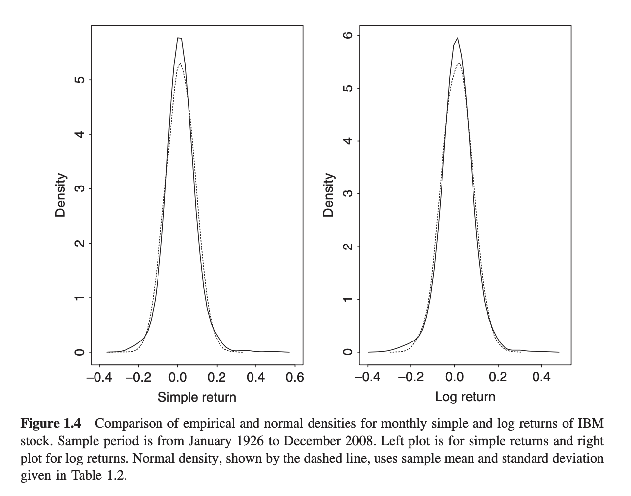
Monthly simple and logarithmic returns of IBM stock with fitted normal distributions. We observe more returns at the extremities of the distributions than the normal distribution would predict. We call these 'fat tails' or 'excess kurtosis'. This image has been taken from 'Analysis of Financial Time Series, 3rd Ed.' by Ruey S. Tsay.

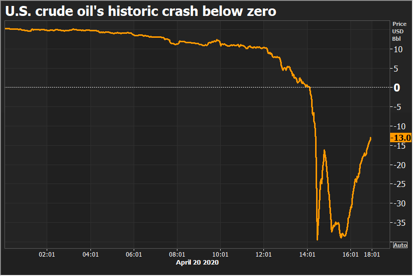
This model also works well because it only permits positive security prices. Securities tend to only have positive prices (although in some cases they can go negative - see the oil crash of 2020).

So, we want a process that generates a series of normally distributed returns $r_t$ - which invites Brownian motion as a natural choice.

Brownian motion

Brownian motion describes the motion of a particle in a fluid or gas. Such a particle bounces around “randomly” within the fluid surrounding it. The path it creates appears quite noisy and random. It can essentially be considered a limiting form of the random walk where both the time between steps and the step length approach zero (with some caveats: namely, if the time step is $t$, the step length must be $\sqrt{t}$ - this produces a process whose variance scales exactly with time). Consider flipping a coin to determine whether to take a step forward or backward. Now let the time between steps approach zero. You would trace a path that looks like this:

1-D Brownian Motion

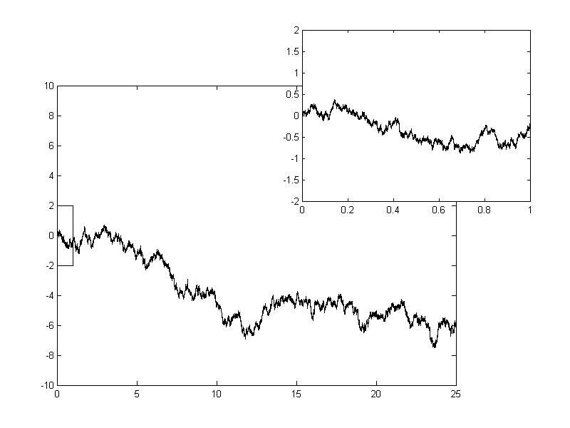
1 dimensional [arithmetic] Brownian motion. Geometric Brownian motion is the exponential of this process. CC BY-SA 3.0, Source

Brownian motion has the very nice property that the trajectories are normally distributed, which is exactly what we are looking for. We can simulate a Brownian process with discrete steps by sampling from a normal distribution (although if you only cared about the terminal value of a time series, you could sample from any distribution with unit variance; due to the central limit theorem the sum of random variables would approach a Gaussian distribution in the long term anyway).

Hence, Brownian motion provides us with the series of normally distributed logarathmic returns $r_t$ as required in $\eqref{eq:rr}$:

$$ \begin{align} r(t) = (\mu-\frac{\sigma^2}{2})t + \sigma B(t) \tag{2} \label{eq:bm} \end{align} $$

Taking the exponential of this process, we’ve recovered an equation for modelling stock price movement.

Of particular interest here is the drift rate $\mu - \frac{\sigma^2}{2}$ which causes the process to drift linearly, as the name suggests. $\mu$ is obvious - it’s the mean continuosly compounding return for the stock, and in the absence of noise (or volatility), the stock price would only grow (or decrease) by this compounding amount. But what about $\frac{\sigma^2}{2}$? Well, it turns out that the expected value of a lognormally distributed variable is $\exp(\mu + \sigma^2/2)$. Since the stock price is lognormally distributed (while returns are normally distributed), and since we require that the expected value of the stock price after continuous compounding to be $S(0)\exp(\mu t)$, we must apply the correction term of $- \frac{\sigma^2}{2}$ to the process.

There’s also a philsophical argument to be made for choosing Brownian motion as the basis for this model. A common assumption made in finance is that markets are efficient, so there should be no arbitrage opportunities. Hence, the market should be unpredictable - if an actor could predict it, that would be an arbitrage opportunity that would be exploited away. Hence, random noise (which is what Brownian motion is, essentially) is a good choice for modelling markets.

Option Pricing

Monte-Carlo simulation is a statistical technique inspired by the casinos of Monaco. Much like gamblers resigning their fates to probability, we hand over the results of statistical analysis to chance. By running enough trials, we can make conclusions with statistical significance.

Consider evaluating a call option with a strike prices of $105 for this stock. What would be the expected value of the option at expiry, given a geometric Brownian model for the stock’s movement? We can estimate this by generating a series of price paths, each of which can be considered a trial. The terminal value of each trial is related to the intrinsic value of the option via the relation $V = \max(0, S - K)$ where $S$ is the stock price and $K$ is the strike price. The mean terminal value provides us with an estimate of the option’s value at expiry, while the standard deviation of terminal values provides us with a measure of how certain we are that the option will expire close to this value.

We can increase the number of trials to increase the statistical certainty of the estimate. Re-running the simulation (by clicking “Regenerate”) on a large number of trials (below) yields a much smaller discrepency between experiments than on a small number of trials (above).

More Advanced Scenarios

Monte-Carlo simulation of terminal values is a relatively simple simulation, and one that is not too useful as this analysis can probably be completed analytically. The true power of Monte-Carlo simulation is unlocked when analysing scenarios that are more difficult to solve analytically, if not impossible. For example, if we wanted to analyse an American-style option, which can be exercised anytime, we might want to count the probability of a stock price exceeding the strike price at any time during the lifetime of that option. We could do this by counting how many trials cross the strike price boundry, which is easy to do with a Monte-Carlo simulation.