Interactive Gradient Descent Demo

November 15, 2021

What is this special algorithm?

Gradient descent is an optimization algorithm for finding the (local) minimum of a function.

Why is that useful?

Say you have some function $f(x,y)$. This function may represent a cost to you, and $x$ and $y$ are some inputs that vary the cost. Naturally, you are going to try to find the values of $x$ and $y$ that minimize the cost. This is a problem of finding the minimum of $f(x,y)$. For example, we may want to find the minimum of this function, which is plotted below:

$$ \begin{align} f(x,y)=3(1 - x)^2 e^{- x^2 - (y + 1)^2} - 10(\frac{x}{5} - x^3 - y^5) e^{-x^2 - y^2} - \frac{1}{3} e^{-(x+1)^2 - y^2} \tag{0} \label{eq:cost_func} \end{align} $$

This is where gradient descent can help.

Why gradient descent?

From elementary calculus, you may remember a procedure for finding the minimum of a function. You could find the first derivative, set it to zero, and solve that equation:

$$ \begin{align} f'(x,y)=0 \tag{1} \label{eq:first_deriv} \end{align} $$

This will reveal the locations of the extrema (maxima and minima) of the function. The sign of the second derivative $f''(x,y)$ can reveal whether the extrema are local maxima or minima. However, solving the first derivative equation $\eqref{eq:first_deriv}$ can be non-trivial, and often require numeric methods. And as your cost function involves higher and higher dimensions, e.g. $f(x,y,z,w,q,u,v,...)$ the problem can become unmanageable. Gradient descent provides an efficient procedure for locating minima by utilizing the first derivative in a clever way.

The gradient descent algorithm

The motivation behind gradient descent is intuitive, and I bet you would arrive at the same procedure in an analogous physical situation. Imagine you find yourself in a thick fog, and you can only see a few feet in front of you and feel the slope of the ground beneath you. You are trying to get to the bottom of a valley as quickly as possible. Surely, you won’t waste your time walking along a flat slope - or worse, head uphill. To descend quickly, you will inspect the slope at your location, and proceed in the direction where the slope is steepest downwards. Gradient is a synonym for slope, hence, you would be performing gradient descent. Conversely, if you were trying to find the top of the hill, you would follow the steepest part of the surface up, wherever you are. This is gradient ascent.

Gradient

Gradient is essentially another word for slope. Most people will be familiar with finding a slope in a 1-dimensional situation. In 1-D, since one can only proceed either forward or backward, the slope is clearly defined. However, in higher dimensions - imagine you find yourself on a hike - the slope may have a different value depending on which direction you go. How does one define the slope at this point?

In vector calculus, one uses the gradient operator $\nabla$, which is a vector of the slopes (or first derivatives) along each dimension.

$$ \begin{align} \nabla f(x,y)= \begin{bmatrix} \frac{\partial f}{dx} (x,y) \\ \frac{\partial f}{dy} (x,y) \end{bmatrix} \tag{2} \label{eq:gradient} \end{align} $$

On a 2D surface defined by $f(x,y)$, this would be the slope along the x-axis and the slope along the y-axis. The slope in any particular direction (which is important, since we are not constrained to move only along either the x-axis or the y-axis) can be found by summing the corresponding x and y components of the slope in that direction. In other words, the dot product of a direction vector with the gradient produces the slope in that direction.

Another interesting property of the gradient is that it gives the direction of the steepest slope. One can see this mathematically - since the slope in any particular direction can be found by dotting that direction vector with the gradient, the dot product is maximized when the gradient is dotted with itself!

Below, I plot the negative gradient of $f(x,y)$ with Mathematica. This gives us the direction of steepest descent at every point on $f$.

Gradient of f

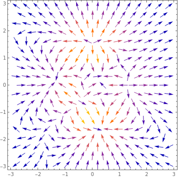
Gradient of f plotted as a vector field.

Follow the steepest part down

Earlier we agreed that if you were blindly navigating down a valley, you would follow the steepest direction of the ground down if you wanted to get to the bottom as quickly as possible. Mathematically, you are traversing down the valley along the gradient at each point, since the gradient vector at each point is the direction of the steepest descent. Looking at the image above, we can see that means following the arrows will lead us to a minimum (but be wary - each minimum has its own basin of attraction! More on that later).

Thus we can define a procedure. It may go something like this:

Inspect the slope at your position and determine the direction of steepest descent
Walk 5 steps in that direction
If you are still descending, go to 1. Otherwise, you’re at the bottom!

You may be wondering how I arrived at 5 steps. Well, it was totally arbitrary. But we can let it be a parameter of our procedure. Let’s call it a descent rate, and assign it the symbol $\alpha$. The larger the descent rate, the less often we’ll have to inspect the slope around us. Computationally, this is more efficient - but as you’ll see, this can lead to pitfalls.

Furthermore, we can make another optimization. When the local slope is still steep, we are probably far from the bottom of the valley. But as the slope gets flatter, we can figure that we are probably approaching the bottom. Hence we may want to descend at a rate proportional to the gradient. Let’s define the gradient with the symbol $\bar{g}$, and redefine our gradient descent procedure:

Inspect the slope at your position and determine the direction of steepest descent
Walk $\alpha \times \|\bar{g}\|$ steps in that direction
If you are still descending, go to 1. Otherwise, you’re at the bottom!

Next, how do we determine if we are still descending? One approach is to check how much we’ve descended on every iteration. If we’re barely changing altitude, then we’re probably essentially at the bottom already.

Mathematically, our procedure looks like:

$$ \begin{align} \bar{p}_{n+1} = \bar{p}_n - \alpha \nabla f(x,y) \tag{3} \label{eq:grad_descent} \end{align} $$

where $p_n$ is our position at the $n^{th}$ iteration of our descent. Try it out on the demo below. Varying the rate $\alpha$ varies the rate of the descent, while varying $X$ and $Y$ vary the initial starting point on the surface. What do you notice?

X 0

Y 0

α 0

Observations

You may notice that gradient descent is sensitive to the initial position. It will pull you towards a local minimum, which may not be the global minimum. The area of the domain that causes gradient descent to converge to a particular minimum is known as that minima’s basin of attraction.

You may also notice that increasing the descent rate $\alpha$ reduces the number of iterations required to arrive at the minimum. But making it too large causes the algorithm to overshoot, and possibly diverge.

Machine learning

You’ve probably heard of gradient descent in the context of machine learning. In that context, the cost function represents the error of our machine learning model. For example, it may be the error of classifying images, and the inputs to the cost function are the weights of the model we are varying. Hence, we can use gradient descent to find the optimal configuration of weights that minimize the classification error of the neural network! In this field, the descent rate $\alpha$ has a special name: it is known as the learning rate. Maybe it’s what our brains have been doing all along.