Blackbox Optimization and Hyperparameter Tuning With Google's Vizier

Automatically and intelligently optimize any kind of system

When you build an machine learning model - or some other kind of algorithmic system - you will have to make choices about the architecture of your system. For example, for a machine learning application, you may need to decide how many neurons to have in a neural network layer, or the rate of gradient descent. Or if you are building a particle filter to track the state of a robot, you may need to choose the shape of a likelihood function. You may be looking for a buffer size and thread count that minimize your use of computing resources. How can you find the optimal architecture for your system?

You could try to find it manually. You can try different values for the number of neurons. You could try different rates of gradient descent. But this process is slow and tedious, and suceptible to pitfalls. Thankfully there exist services that can optimize your system for you, in an intelligent and efficient way.

Introducing Vizier

Vizier is an optimization service created at Google for blackbox and hyperparameter optimization. It can be used to optimize any kind of system as long as you can pass inputs to the system - that are suggested by Vizier - and get outputs from the system - metrics that Vizier is trying to optimize, such as by maximizing or minimizing them. The system itself is treated as a blackbox.

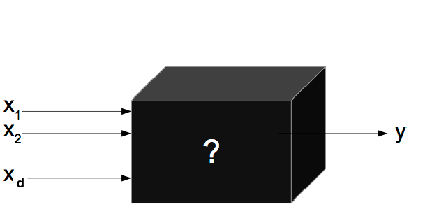
Blackbox optimization doesn't requre any understanding of the system itself, as long as you can pass inputs and get outputs. Source: Per Instance Algorithm Configuration for Continuous Black Box Optimization - Scientific Figure on ResearchGate. Available from: https://www.researchgate.net/figure/black-box-Optimization_fig1_322035981 [accessed 23 Feb, 2023]

Unlike non-blackbox optimization systems such as gradient descent which require an understanding of the relationship between the parameters of the system and the metric being minimized or maximized, a blackbox system like Vizier does not require any insight into the system itself. It can still search the parameter space efficiently for you, and find the values of the parameters that optimize your system. This also makes it more robust to complex, discontinuous and non-convex metric functions.

Parameters vs Hyperparameters

Aside: the distinction comes from machine learning applications, where “parameters” are considered the values inside the model used for inference and found through training on a dataset, while hyperparameters describe the architecture of the model or the training procedure. However, a blackbox optimization service like Vizier can be used to optimize any kind of system, but it won’t be an efficient way of training a machine learning model. But it is a good way to optimize the architecture of the model.

An Example

I am going to use an example that is not machine learning related, but still demonstrates the power and simplicity of a blackbox optimization algorithm such as Vizier. Say we have a noisy signal like the one below:

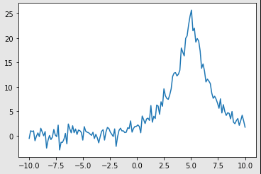
Some noisy signal.

Let’s try to find an analytical function that fits this signal. We can’t decide if we want to fit a Gaussian or Laplace function to the signal, and both functions have their own parameters - such as mean and variance - that we are also trying to estimate.

As long as we can give Vizier a metric we are trying to optimize, it will find an optimal function for us.

Setting Up The Problem

The first parameter we want to search is the model type: Gaussian or Laplace:

{
    'parameter_id': 'model',
    'categorical_value_spec' : {
        'values': [
            'gaussian',
            'laplace',
        ]
}

But each model has its own set of parameters that defines its shape. Let’s call these “child parameters” of each model.

For the Gaussian, these are the mean mu (\(\mu\)) and standard deviation sigma (\(\sigma\)).

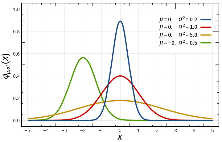
Gaussian distribution with parameters mu and sigma. Taken from: https://commons.wikimedia.org/wiki/File:Normal_Distribution_PDF.svg

For the Laplace - the notation depends on the literature - but generally there is the location parameter or mean mu (\(\mu\)) and scale factor b (\(b\)).

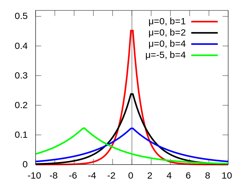
Laplace distribution with parameters mu and b. Taken from: https://commons.wikimedia.org/wiki/File:Laplace_pdf_mod.svg

For disambiguity from the mean of the Gaussian, let’s refer to the location parameter of the Laplace distribution as a instead of mu.

When trying to fit the Gaussian distribution, we don’t want Vizier to try to estimate the parameters of the Laplace distribution and vice versa. Luckily we can specify the parameters of each distribution as child, or conditional, parameters of the parent model parameter:

'conditional_parameter_specs': [
{
    "parameter_spec": {
        "parameter_id": "mu",
        "scale_type": 'UNIT_LINEAR_SCALE',
        "double_value_spec": {
        "min_value": 0,
        "max_value": 10.0,
        },
    },
    "parent_categorical_values": {
        "values": ['gaussian']
    }
},
{
    "parameter_spec": {
        "parameter_id": "sigma",
        "scale_type": 'UNIT_LINEAR_SCALE',
        "double_value_spec": {
        "min_value": 1e-1,
        "max_value": 5.0,
        },
    },
    "parent_categorical_values": {
        "values": ['gaussian']
    }
},
    {
    "parameter_spec": {
        "parameter_id": "a",
        "scale_type": 'UNIT_LINEAR_SCALE',
        "double_value_spec": {
        "min_value": 0,
        "max_value": 10.0,
        },
    },
    "parent_categorical_values": {
        "values": ['laplace']
    }
},
{
    "parameter_spec": {
        "parameter_id": "b",
        "scale_type": 'UNIT_LINEAR_SCALE',
        "double_value_spec": {
        "min_value": 1e-1,
        "max_value": 5.0,
        },
    },
    "parent_categorical_values": {
        "values": ['laplace']
    }
}]

Lastly, we need to define the metric that Vizier will be to optimizing. I want to fit a function to the signal as closely as possible, and I will evaluate how well it fits the signal by calculating the sum of squares of residuals between the analytical function and the data. The smaller this number, the better the fit. All we need to tell Vizier is that there is this metric we are trying to minimize:

metric_ssr = {
    'metric_id': 'sum_of_squared_residuals',
    'goal': 'MINIMIZE',
}

We put all of this together and that defines our problem:

study = {
    'display_name': 'vizier_experiment',
    'study_spec' :
    {
        'parameters': [param_model],
        'metrics': [metric_ssr]
    }
}

Note that Vizier has no understanding of the parameters themselves. Gaussian and Laplace are simply types of a categorical parameter, and to Vizier have no meaning besides that. They are given meaning by my code that consumes them, but to Vizier, that code lives in a blackbox. I’m leaving out the code for brevity, but you can find it all at the link at the end of the article to see what I mean.

Searching

For each trial, Vizier suggests a set of parameters for us to try. We evaluate how well these parameters work ourselves, calculate the metric (the sum of squared residuals) and return the result of the metric evaluation to Vizier. Vizier uses the result to generate the next set of parameters to try.

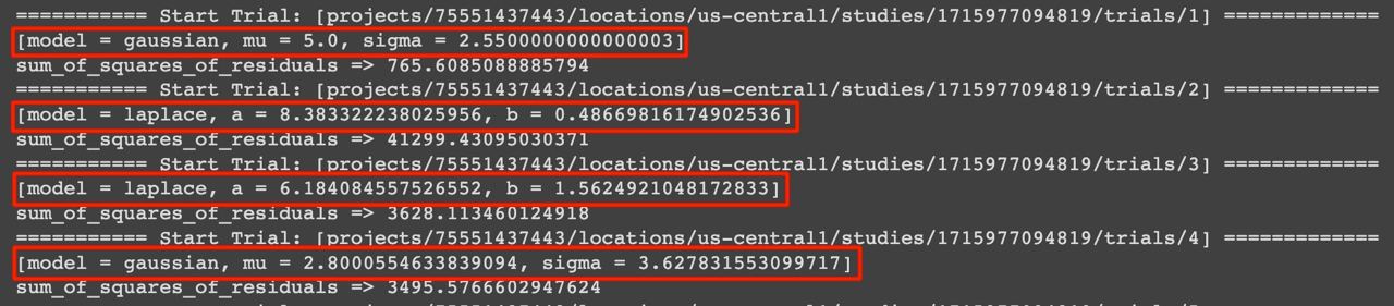
Vizier suggesting parameters for trials.

Notice that Vizier only suggests Gaussian parameters when the model is Gaussian, and vice versa for the Laplace model.

How does Vizier search for optimal parameters? It can do a grid or random search, but the real magic is the combination of other algorithms it employs: Gaussian process bandits, linear combination search, or their variants.

Via GCP we can check these cool charts of Vizier’s progress:

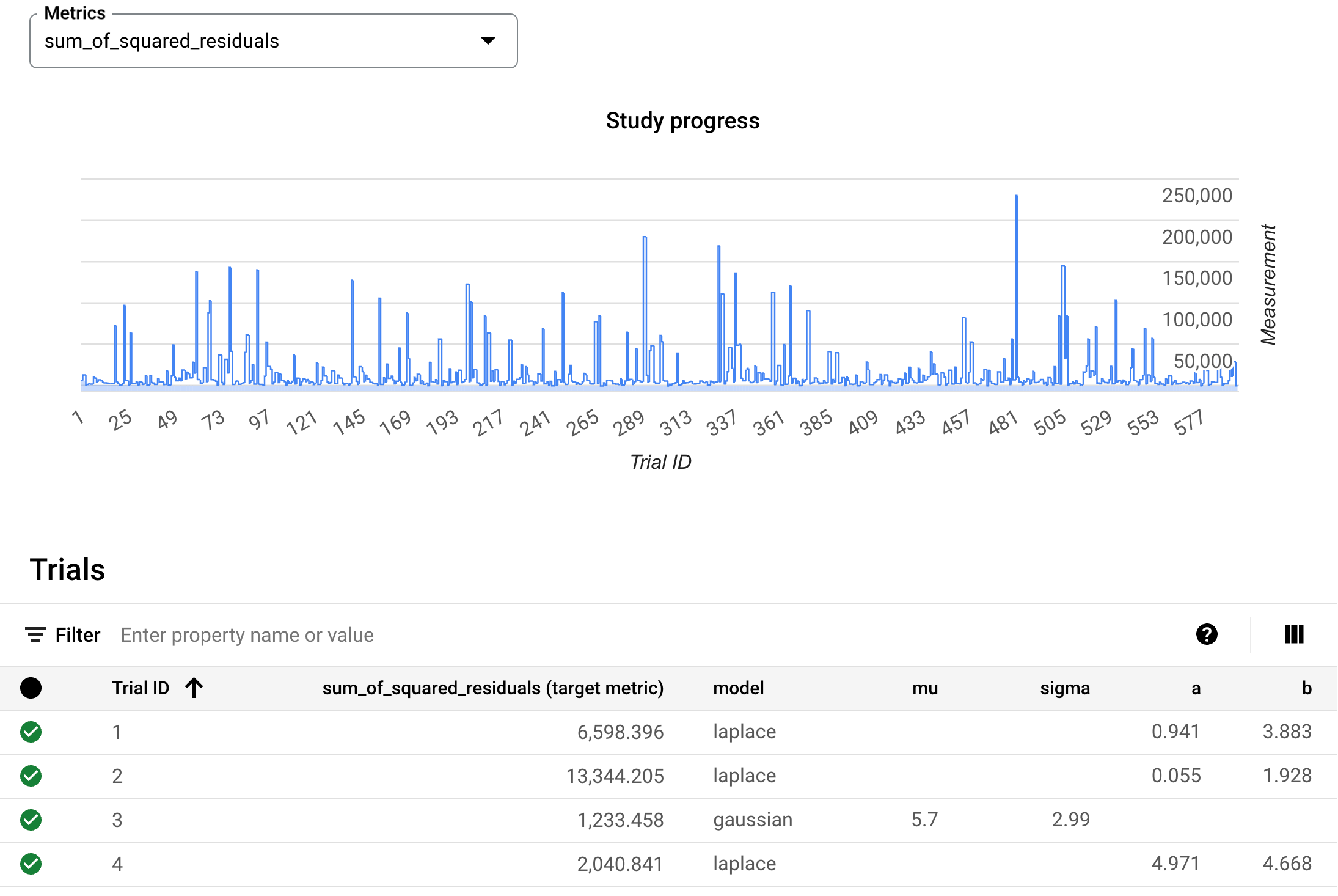
A study table showing the evolution of the metric being optimized and the parameters of each trial.

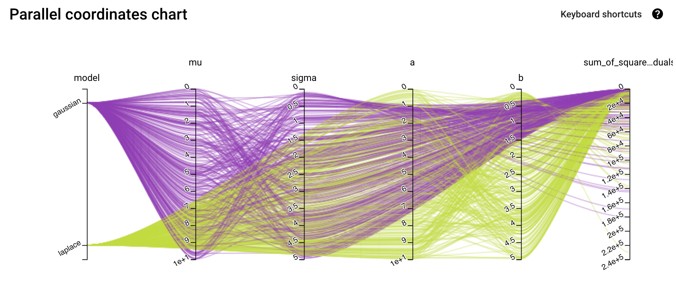
A parallel chart showing the sets of parameters attempted and the resulting metric value.

Optimized Fit

We can see that the Laplace distribution slightly wins out over the Gaussian:

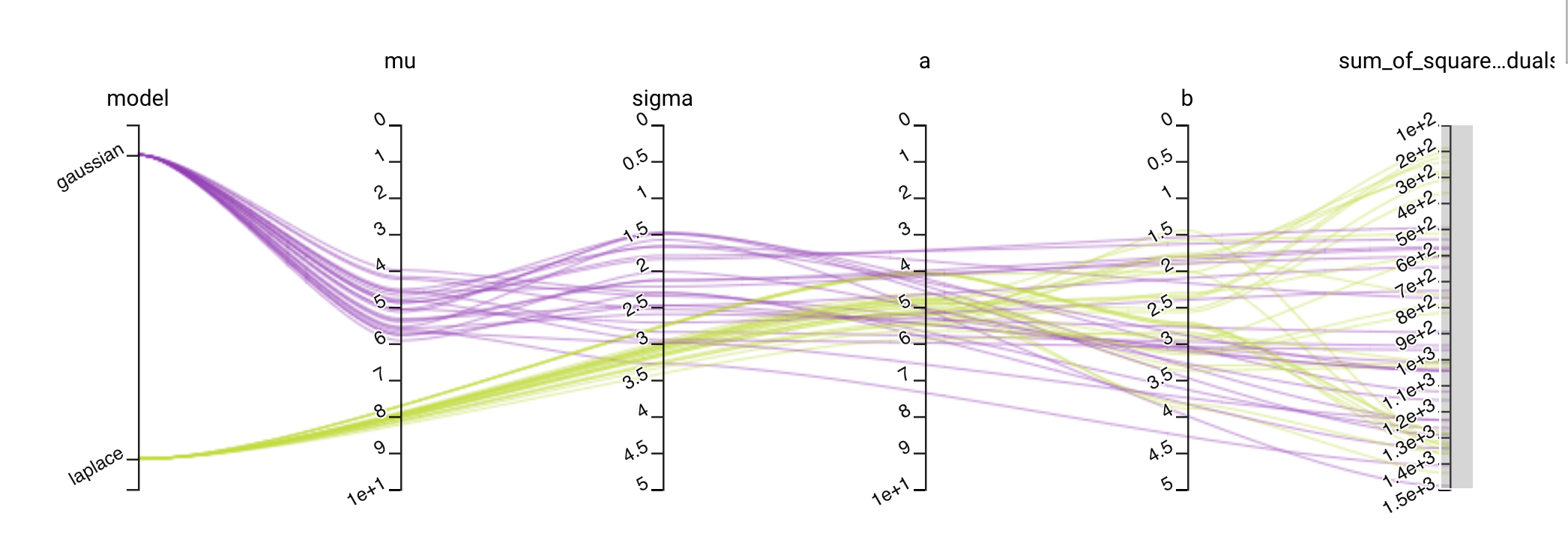
Parallel chart zoomed in to show the top trials that minimize the sum of squared residuals. A better fit is found with a Laplace distribution than a Gaussian distribution.

We query Vizier for the optimal trial parameters and plot them:

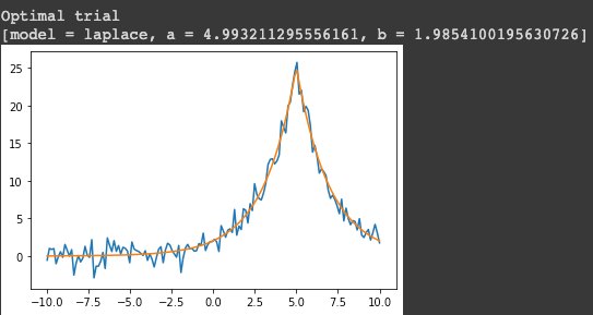
Optimized parameters that fit the noisy signal.

It’s almost a perfect fit! The parameters Vizier found are close to the parameters I used to generate the signal before adding noise: a Laplace distribution with \(a=5\) and \(b=2\).

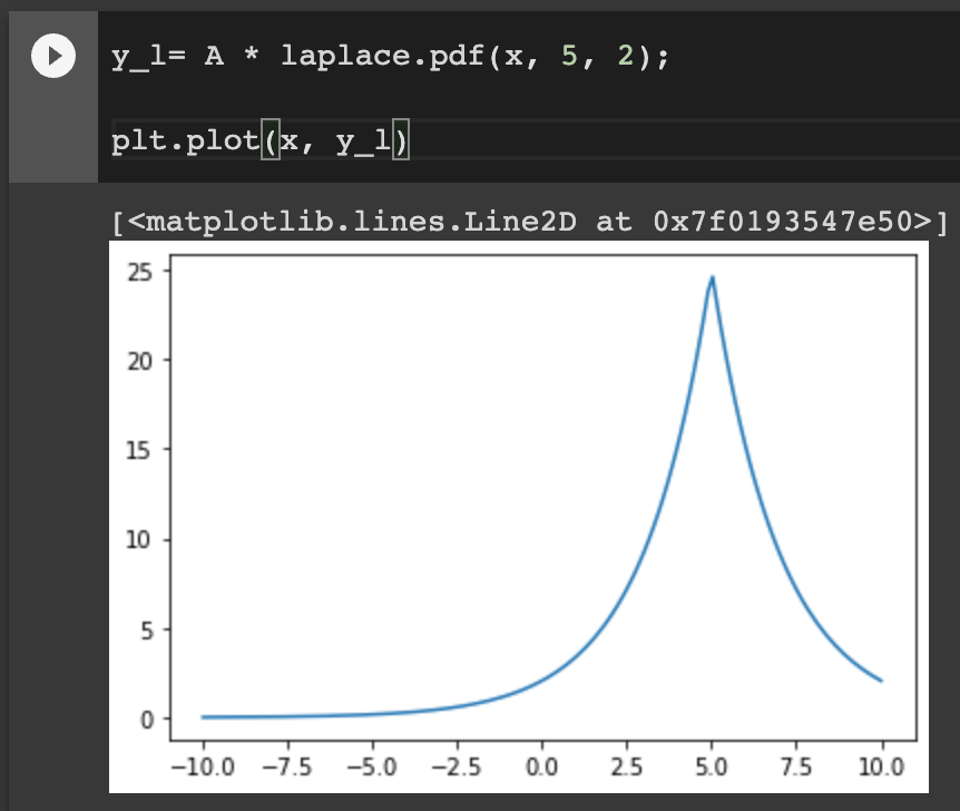
Original Laplace signal.

For comparison, a Gaussian would have a rounder peak and thinner tails.

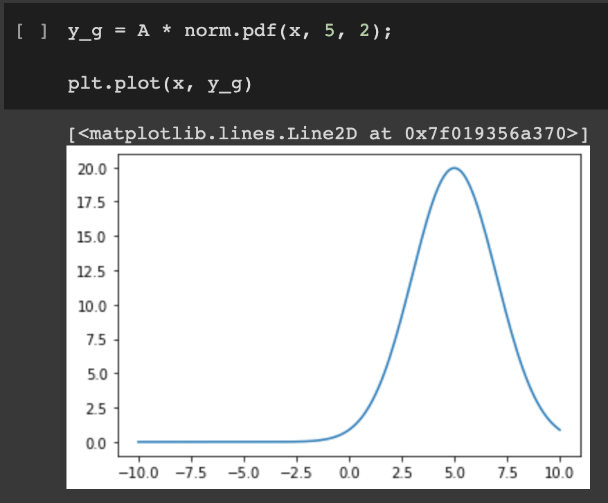
A comparative Gaussian distribution.

How Can I Reproduce This?

The colab I used to generate this article can be found here. I used GCP’s Vertex AI Vizier API because it generates some cool charts like the ones I included in this post, but be aware it can be expensive ($1/trial). Vizier is also open-source and available here.